From Neurons to Gradients: Unpacking FastAI Lesson 3

Introduction

Hey there, fellow data adventurers! 👋 It’s been a couple of week since my last post - blame exams and and obsessive quest to tweak every configuration setting for my workflow (which is turned into a week-long habit hole - i regret nothing). But today, I’m excited to dive back into the world of AI and share my latest escapades from Lesson 3 of the FastAI course taught by the indomitable Jeremy Horawd. Spoiler alert: it’s packed with enough neural wonders to make your brain do a happy dance.🕺

In the coming post, I’ll guide you through:

• Picking of right AI model that’s just right for you
• Dissecting the anatomy of these models (paramedics not required)🧬
• The inner workings of neuron networks 🧠
• The Titanic competition

So, hold onto your neural nets and let’s jump right into it, shall we?

Choosing the Right Model: A Guide to Navigating the Neural Jungle

Alright folks, buckle up! We’re diving into the exhilarating world of choosing the perfect image model. It’s like shopping for a new gadget: you want something sleek, efficient, and most importantly - something that get the job done without draining your power (or breaking the bank),

I’m going to guide you through the hands-on example to illustrate the difference between two popular image models. So, let’s play around with training a pet detector model, shall we?

First things first, let’s get our setup ready:

from fastai.vision.all import *
import timm

path = untar_data(URLs.PETS)/'images'


dls = ImageDataLoaders.from_name_func(
    ".",
    get_image_files(path),
    valid_pct=0.2,
    seed=42,
    label_func=RegexLabeller(pat=r'^([^/]+)_\d+'),
    item_tfms=Resize(224)
)

100.00% [811712512/811706944 01:13<00:00]

Lemme break down what’s happening here. We’re using The Oxford-IIIT Pet dataset, fetched with a nifty little URL constant provide by FastAI. If you’re staring at the pattern pat=r'^([^/]+)\_\d+' like it’s some alien script, fear not! It’s just a regular expression used to extract label from filenames using fastai RegexLabeller

Here’s the cheat sheet for the pattern:

• ^ asserts the start of a string.
• ([^/]+) matches one or more characters that are not forward slash and captures them as a group.
• _ matches an underscore.
• \d+ matches one ore more digits.

Now, let’s visualize our data:

dls.show_batch(max_n=4)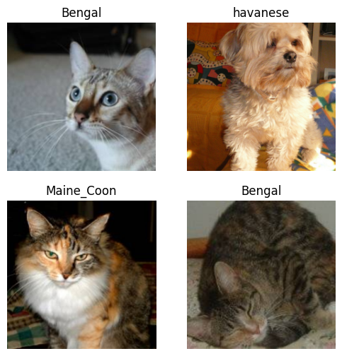

And, it’s training time! We start with a ResNet34 architecture:

learn = vision_learner(dls, resnet34, metrics=error_rate)
learn.fine_tune(3)

Downloading: "https://download.pytorch.org/models/resnet34-b627a593.pth" to /root/.cache/torch/hub/checkpoints/resnet34-b627a593.pth

100%|██████████| 83.3M/83.3M [00:00<00:00, 147MB/s] 

epoch	train_loss	valid_loss	error_rate	time
0	1.491942	0.334319	0.105548	00:26

epoch	train_loss	valid_loss	error_rate	time
0	0.454661	0.367568	0.112991	00:32
1	0.272869	0.274704	0.081867	00:33
2	0.144361	0.246424	0.073072	00:33

Alright after about 2 minutes, we hit a 7% error rate. Not too shabby! But here’s the catch: ResNet34 is like the reliable old family car of neuron networks - good but not the fastest on the block. to spice thing up, we need to find a better, more turbo-changed model🏎️

Time to Upgrade: Diving into the Model Jungle

There are zillion architectures in the Pytorch image model library - ok, maybe not a zillion, but a lot! Most are mathematical functions like RELUs(Rectified Linear Units), which we’ll get into shortly. So, which model should we choose? It boil down to three things:

1. Speed
2. Memory Usage
3. Accuracy

The “Which Image Model is Best?” Notebook

Check out this gem by Jeremy Howard: Which image models are best. It’s a treasure trove for finding the perfect architecture, and i highly recommend you go to his notebook read it and you should totally upvote it because Jeremy rocks.

i just copy the plot into here for so you can look at that quickly (but remember to give him a upvote).

Plotly = require('https://cdn.plot.ly/plotly-latest.min.js');
df_results = FileAttachment("results-imagenet.csv").csv()
df = FileAttachment("benchmark-infer-amp-nhwc-pt111-cu113-rtx3090.csv").csv()

df_merged = {
  let df_results_processed = df_results.map(r => ({ ...r, model_org: r.model, model: r.model.split('.')[0] }));

  const dfColumns = Object.keys(df[0]);
  const dfResultsColumns = Object.keys(df_results_processed[0]);

  return df.flatMap(d => {
    const matches = df_results_processed.filter(r => r.model === d.model);
    return matches.map(match => {
      let mergedRow = {};
      dfColumns.forEach(col => {
        if (dfResultsColumns.includes(col) && col !== 'model') { mergedRow[`${col}_x`] = d[col]; } else { mergedRow[col] = d[col]; }
      });
      dfResultsColumns.forEach(col => {
        if (dfColumns.includes(col) && col !== 'model') { mergedRow[`${col}_y`] = match[col]; } else { mergedRow[col] = match[col]; }
      });
      return mergedRow;
    });
  });
}

df_final = df_merged
  .map(d => ({...d, secs: 1 / Number(d.infer_samples_per_sec)}))
  .map(d => {
    const familyMatch = d.model.match(/^([a-z]+?(?:v2)?)(?:\d|_|$)/);
    let family = familyMatch ? familyMatch[1] : '';
    if (d.model.includes('in22')) family += '_in22';
    if (d.model.match(/resnet.*d/)) family += 'd';
    return {...d, family: family};
  })
  .filter(d => !d.model.endsWith('gn'))
  .filter(d => /^re[sg]netd?|beit|convnext|levit|efficient|vit|vgg|swin/.test(d.family));
{
  const uniqueFamilies = [...new Set(df_final.map(d => d.family))];
  const colorScale = uniqueFamilies.map((family, index) => { return `hsl(${index * 360 / uniqueFamilies.length}, 70%, 50%)`; });
  const traces = uniqueFamilies.map((family, index) => {
    const familyData = df_final.filter(d => d.family === family);
    return {
      name: family,
      x: familyData.map(d => d.secs),
      y: familyData.map(d => Number(d.top1)),
      mode: 'markers',
      type: 'scatter',
      marker: { size: familyData.map(d => Math.pow(Number(d.infer_img_size), 2) / 5700), color: colorScale[index], },
      text: familyData.map(d => `${d.model}<br> family=${d.family}<br> secs=${d.secs.toFixed(8)}<br> top1=${Number(d.top1).toFixed(3)}<br> size=${d.param_count_x}<br> infer_img_size=${d.infer_img_size}`),
      hoverinfo: 'text',
      hoverlabel: { bgcolor: colorScale[index] }
    };
  });
  const layout = {
    title: 'Inference',
    width: 1000,
    height: 800,
    xaxis: { title: 'secs', type: 'log', autorange: true, gridcolor: 'rgb(233,233,233)', },
    yaxis: { title: 'top1', range: [65, 90], gridcolor: 'rgb(233,233,233)', },
    plot_bgcolor: 'rgb(240,240,255)',
    showlegend: true,
    legend: { title: {text: 'family'}, itemclick: 'toggle', itemdoubleclick: 'toggleothers' },
    hovermode: 'closest'
  };
  const config = {responsive: true};
  const plot = DOM.element('div');
  Plotly.newPlot(plot, traces, layout, config);
  return plot;
}

Here’s the plot breakdown from the notebook:

• The X-axis shows seconds per sample(how fast it is) - to the left is better.
• The Y-axis shows accuracy - higher is better.

Ideally, you want models that hover around the top left corner. We often use ResNet34 because it’s like the comfortable pair of jeans everyone swears by. But it’s not the cutting-edge model anymore. Let’s explore something better: ConvNeXT models! 🎉

First, make sure you install the timm via pip or conda:

pip install timm

or

conda install timm

Then, let’s search for all the ConvNext models:

timm.list_models("convnext*")

['convnext_atto',
 'convnext_atto_ols',
 'convnext_base',
 'convnext_femto',
 'convnext_femto_ols',
 'convnext_large',
 'convnext_large_mlp',
 'convnext_nano',
 'convnext_nano_ols',
 'convnext_pico',
 'convnext_pico_ols',
 'convnext_small',
 'convnext_tiny',
 'convnext_tiny_hnf',
 'convnext_xlarge',
 'convnext_xxlarge',
 'convnextv2_atto',
 'convnextv2_base',
 'convnextv2_femto',
 'convnextv2_huge',
 'convnextv2_large',
 'convnextv2_nano',
 'convnextv2_pico',
 'convnextv2_small',
 'convnextv2_tiny']

Found one? Awesome! Now, let’s put it to the test. We’ll specify the architecture as a string when we call vision_learner, Why previous time when we use ResNet34 we don’t need to pass it as string? you say! That’s because ResNet34 was built in fastai library so you just need to call it but with ConvNext you have to pass the arch as a string for it to work, alright let’s see what it look like:

arch = 'convnext_tiny.fb_in22k'
learn = vision_learner(dls, arch, metrics=error_rate).to_fp16()
learn.fine_tune(3)

epoch	train_loss	valid_loss	error_rate	time
0	1.123377	0.240116	0.081191	00:27

epoch	train_loss	valid_loss	error_rate	time
0	0.260218	0.225793	0.071719	00:34
1	0.199426	0.169573	0.059540	00:33
2	0.132157	0.166686	0.056834	00:33

Results Are In!

Training time goes up a little bit like 3, 4 seconds. But, and here’s the kicker - the accuracy jumps from 7.3% error down to 5.6%!🚀

The model names might looks cryptic. Here’s the decoder ring:

• Tiny, small, large. etc.: Size and resource demands.
• fb_in22k: Trained on ImageNet dataset with 22,000 image categories by Facebook AI Research(FAIR)

These ConvNeXT models generally outperform others in terms of accuracy on standard photos of natural objects. So, there you have it! We’ve seen how to choose and implement a better architecture for your image models. Remember, it’s all about finding the right balance between speed, memory, and accuracy. Stay tuned, as we’ll tackle deeper intricacies of neural networks next 🎢

What’s in the Model?

Alright, you see? Our model did better, right? Now, you’ve probably wondering, how do we turn this awesome piece of neural magic into an actual application? They key is to save the trained model so that users won’t have to wait for the training time.

To do that, we export our learner with the following command, creating a magical file called model.pkl:

learn.export('model.pkl')

For those of you who’ve stuck around through my previous blog posts, you’ll remember that when i deploy an application on HuggingFace Spaces, I simply load this model.pkl file. This way, the learner operates almost exactly like the trained learn object, but it’s really instantly means no more waiting for eons!

Now, you might be scratching your head, wondering. “what did we just do exactly? What inside this model.pkl file?”

Dissecting the model.pkl File

Alright, grab your virtual scalpel, because we’re doing some model surgery! The model.pkl file is essentially a saved learner, and it houses two main things:

1. Pre-processing Steps: This includes all the steps needed to turn your raw images into something model can understand. Essentially, this is the information your DataLoaders(dls), DataBlock, or any other pre-processing pipeline you’ve set up.
2. The Trained Model: This is the most crucial part - a model that has been trained and is ready to make predictions.

To peek inside, we can load the model back up and check it out:

m = learn.model
m

Sequential(
  (0): TimmBody(
    (model): ConvNeXt(
      (stem): Sequential(
        (0): Conv2d(3, 96, kernel_size=(4, 4), stride=(4, 4))
        (1): LayerNorm2d((96,), eps=1e-06, elementwise_affine=True)
      )
      (stages): Sequential(
        (0): ConvNeXtStage(
          (downsample): Identity()
          (blocks): Sequential(
            (0): ConvNeXtBlock(
              (conv_dw): Conv2d(96, 96, kernel_size=(7, 7), stride=(1, 1), padding=(3, 3), groups=96)
              (norm): LayerNorm((96,), eps=1e-06, elementwise_affine=True)
              (mlp): Mlp(
                (fc1): Linear(in_features=96, out_features=384, bias=True)
                (act): GELU()
                (drop1): Dropout(p=0.0, inplace=False)
                (norm): Identity()
                (fc2): Linear(in_features=384, out_features=96, bias=True)
                (drop2): Dropout(p=0.0, inplace=False)
              )
              (shortcut): Identity()
              (drop_path): Identity()
            )
            (1): ConvNeXtBlock(
              (conv_dw): Conv2d(96, 96, kernel_size=(7, 7), stride=(1, 1), padding=(3, 3), groups=96)
              (norm): LayerNorm((96,), eps=1e-06, elementwise_affine=True)
              (mlp): Mlp(
                (fc1): Linear(in_features=96, out_features=384, bias=True)
                (act): GELU()
                (drop1): Dropout(p=0.0, inplace=False)
                (norm): Identity()
                (fc2): Linear(in_features=384, out_features=96, bias=True)
                (drop2): Dropout(p=0.0, inplace=False)
              )
              (shortcut): Identity()
              (drop_path): Identity()
            )
            (2): ConvNeXtBlock(
              (conv_dw): Conv2d(96, 96, kernel_size=(7, 7), stride=(1, 1), padding=(3, 3), groups=96)
              (norm): LayerNorm((96,), eps=1e-06, elementwise_affine=True)
              (mlp): Mlp(
                (fc1): Linear(in_features=96, out_features=384, bias=True)
                (act): GELU()
                (drop1): Dropout(p=0.0, inplace=False)
                (norm): Identity()
                (fc2): Linear(in_features=384, out_features=96, bias=True)
                (drop2): Dropout(p=0.0, inplace=False)
              )
              (shortcut): Identity()
              (drop_path): Identity()
            )
          )
        )
        (1): ConvNeXtStage(
          (downsample): Sequential(
            (0): LayerNorm2d((96,), eps=1e-06, elementwise_affine=True)
            (1): Conv2d(96, 192, kernel_size=(2, 2), stride=(2, 2))
          )
          (blocks): Sequential(
            (0): ConvNeXtBlock(
              (conv_dw): Conv2d(192, 192, kernel_size=(7, 7), stride=(1, 1), padding=(3, 3), groups=192)
              (norm): LayerNorm((192,), eps=1e-06, elementwise_affine=True)
              (mlp): Mlp(
                (fc1): Linear(in_features=192, out_features=768, bias=True)
                (act): GELU()
                (drop1): Dropout(p=0.0, inplace=False)
                (norm): Identity()
                (fc2): Linear(in_features=768, out_features=192, bias=True)
                (drop2): Dropout(p=0.0, inplace=False)
              )
              (shortcut): Identity()
              (drop_path): Identity()
            )
            (1): ConvNeXtBlock(
              (conv_dw): Conv2d(192, 192, kernel_size=(7, 7), stride=(1, 1), padding=(3, 3), groups=192)
              (norm): LayerNorm((192,), eps=1e-06, elementwise_affine=True)
              (mlp): Mlp(
                (fc1): Linear(in_features=192, out_features=768, bias=True)
                (act): GELU()
                (drop1): Dropout(p=0.0, inplace=False)
                (norm): Identity()
                (fc2): Linear(in_features=768, out_features=192, bias=True)
                (drop2): Dropout(p=0.0, inplace=False)
              )
              (shortcut): Identity()
              (drop_path): Identity()
            )
            (2): ConvNeXtBlock(
              (conv_dw): Conv2d(192, 192, kernel_size=(7, 7), stride=(1, 1), padding=(3, 3), groups=192)
              (norm): LayerNorm((192,), eps=1e-06, elementwise_affine=True)
              (mlp): Mlp(
                (fc1): Linear(in_features=192, out_features=768, bias=True)
                (act): GELU()
                (drop1): Dropout(p=0.0, inplace=False)
                (norm): Identity()
                (fc2): Linear(in_features=768, out_features=192, bias=True)
                (drop2): Dropout(p=0.0, inplace=False)
              )
              (shortcut): Identity()
              (drop_path): Identity()
            )
          )
        )
        (2): ConvNeXtStage(
          (downsample): Sequential(
            (0): LayerNorm2d((192,), eps=1e-06, elementwise_affine=True)
            (1): Conv2d(192, 384, kernel_size=(2, 2), stride=(2, 2))
          )
          (blocks): Sequential(
            (0): ConvNeXtBlock(
              (conv_dw): Conv2d(384, 384, kernel_size=(7, 7), stride=(1, 1), padding=(3, 3), groups=384)
              (norm): LayerNorm((384,), eps=1e-06, elementwise_affine=True)
              (mlp): Mlp(
                (fc1): Linear(in_features=384, out_features=1536, bias=True)
                (act): GELU()
                (drop1): Dropout(p=0.0, inplace=False)
                (norm): Identity()
                (fc2): Linear(in_features=1536, out_features=384, bias=True)
                (drop2): Dropout(p=0.0, inplace=False)
              )
              (shortcut): Identity()
              (drop_path): Identity()
            )
            (1): ConvNeXtBlock(
              (conv_dw): Conv2d(384, 384, kernel_size=(7, 7), stride=(1, 1), padding=(3, 3), groups=384)
              (norm): LayerNorm((384,), eps=1e-06, elementwise_affine=True)
              (mlp): Mlp(
                (fc1): Linear(in_features=384, out_features=1536, bias=True)
                (act): GELU()
                (drop1): Dropout(p=0.0, inplace=False)
                (norm): Identity()
                (fc2): Linear(in_features=1536, out_features=384, bias=True)
                (drop2): Dropout(p=0.0, inplace=False)
              )
              (shortcut): Identity()
              (drop_path): Identity()
            )
            (2): ConvNeXtBlock(
              (conv_dw): Conv2d(384, 384, kernel_size=(7, 7), stride=(1, 1), padding=(3, 3), groups=384)
              (norm): LayerNorm((384,), eps=1e-06, elementwise_affine=True)
              (mlp): Mlp(
                (fc1): Linear(in_features=384, out_features=1536, bias=True)
                (act): GELU()
                (drop1): Dropout(p=0.0, inplace=False)
                (norm): Identity()
                (fc2): Linear(in_features=1536, out_features=384, bias=True)
                (drop2): Dropout(p=0.0, inplace=False)
              )
              (shortcut): Identity()
              (drop_path): Identity()
            )
            (3): ConvNeXtBlock(
              (conv_dw): Conv2d(384, 384, kernel_size=(7, 7), stride=(1, 1), padding=(3, 3), groups=384)
              (norm): LayerNorm((384,), eps=1e-06, elementwise_affine=True)
              (mlp): Mlp(
                (fc1): Linear(in_features=384, out_features=1536, bias=True)
                (act): GELU()
                (drop1): Dropout(p=0.0, inplace=False)
                (norm): Identity()
                (fc2): Linear(in_features=1536, out_features=384, bias=True)
                (drop2): Dropout(p=0.0, inplace=False)
              )
              (shortcut): Identity()
              (drop_path): Identity()
            )
            (4): ConvNeXtBlock(
              (conv_dw): Conv2d(384, 384, kernel_size=(7, 7), stride=(1, 1), padding=(3, 3), groups=384)
              (norm): LayerNorm((384,), eps=1e-06, elementwise_affine=True)
              (mlp): Mlp(
                (fc1): Linear(in_features=384, out_features=1536, bias=True)
                (act): GELU()
                (drop1): Dropout(p=0.0, inplace=False)
                (norm): Identity()
                (fc2): Linear(in_features=1536, out_features=384, bias=True)
                (drop2): Dropout(p=0.0, inplace=False)
              )
              (shortcut): Identity()
              (drop_path): Identity()
            )
            (5): ConvNeXtBlock(
              (conv_dw): Conv2d(384, 384, kernel_size=(7, 7), stride=(1, 1), padding=(3, 3), groups=384)
              (norm): LayerNorm((384,), eps=1e-06, elementwise_affine=True)
              (mlp): Mlp(
                (fc1): Linear(in_features=384, out_features=1536, bias=True)
                (act): GELU()
                (drop1): Dropout(p=0.0, inplace=False)
                (norm): Identity()
                (fc2): Linear(in_features=1536, out_features=384, bias=True)
                (drop2): Dropout(p=0.0, inplace=False)
              )
              (shortcut): Identity()
              (drop_path): Identity()
            )
            (6): ConvNeXtBlock(
              (conv_dw): Conv2d(384, 384, kernel_size=(7, 7), stride=(1, 1), padding=(3, 3), groups=384)
              (norm): LayerNorm((384,), eps=1e-06, elementwise_affine=True)
              (mlp): Mlp(
                (fc1): Linear(in_features=384, out_features=1536, bias=True)
                (act): GELU()
                (drop1): Dropout(p=0.0, inplace=False)
                (norm): Identity()
                (fc2): Linear(in_features=1536, out_features=384, bias=True)
                (drop2): Dropout(p=0.0, inplace=False)
              )
              (shortcut): Identity()
              (drop_path): Identity()
            )
            (7): ConvNeXtBlock(
              (conv_dw): Conv2d(384, 384, kernel_size=(7, 7), stride=(1, 1), padding=(3, 3), groups=384)
              (norm): LayerNorm((384,), eps=1e-06, elementwise_affine=True)
              (mlp): Mlp(
                (fc1): Linear(in_features=384, out_features=1536, bias=True)
                (act): GELU()
                (drop1): Dropout(p=0.0, inplace=False)
                (norm): Identity()
                (fc2): Linear(in_features=1536, out_features=384, bias=True)
                (drop2): Dropout(p=0.0, inplace=False)
              )
              (shortcut): Identity()
              (drop_path): Identity()
            )
            (8): ConvNeXtBlock(
              (conv_dw): Conv2d(384, 384, kernel_size=(7, 7), stride=(1, 1), padding=(3, 3), groups=384)
              (norm): LayerNorm((384,), eps=1e-06, elementwise_affine=True)
              (mlp): Mlp(
                (fc1): Linear(in_features=384, out_features=1536, bias=True)
                (act): GELU()
                (drop1): Dropout(p=0.0, inplace=False)
                (norm): Identity()
                (fc2): Linear(in_features=1536, out_features=384, bias=True)
                (drop2): Dropout(p=0.0, inplace=False)
              )
              (shortcut): Identity()
              (drop_path): Identity()
            )
          )
        )
        (3): ConvNeXtStage(
          (downsample): Sequential(
            (0): LayerNorm2d((384,), eps=1e-06, elementwise_affine=True)
            (1): Conv2d(384, 768, kernel_size=(2, 2), stride=(2, 2))
          )
          (blocks): Sequential(
            (0): ConvNeXtBlock(
              (conv_dw): Conv2d(768, 768, kernel_size=(7, 7), stride=(1, 1), padding=(3, 3), groups=768)
              (norm): LayerNorm((768,), eps=1e-06, elementwise_affine=True)
              (mlp): Mlp(
                (fc1): Linear(in_features=768, out_features=3072, bias=True)
                (act): GELU()
                (drop1): Dropout(p=0.0, inplace=False)
                (norm): Identity()
                (fc2): Linear(in_features=3072, out_features=768, bias=True)
                (drop2): Dropout(p=0.0, inplace=False)
              )
              (shortcut): Identity()
              (drop_path): Identity()
            )
            (1): ConvNeXtBlock(
              (conv_dw): Conv2d(768, 768, kernel_size=(7, 7), stride=(1, 1), padding=(3, 3), groups=768)
              (norm): LayerNorm((768,), eps=1e-06, elementwise_affine=True)
              (mlp): Mlp(
                (fc1): Linear(in_features=768, out_features=3072, bias=True)
                (act): GELU()
                (drop1): Dropout(p=0.0, inplace=False)
                (norm): Identity()
                (fc2): Linear(in_features=3072, out_features=768, bias=True)
                (drop2): Dropout(p=0.0, inplace=False)
              )
              (shortcut): Identity()
              (drop_path): Identity()
            )
            (2): ConvNeXtBlock(
              (conv_dw): Conv2d(768, 768, kernel_size=(7, 7), stride=(1, 1), padding=(3, 3), groups=768)
              (norm): LayerNorm((768,), eps=1e-06, elementwise_affine=True)
              (mlp): Mlp(
                (fc1): Linear(in_features=768, out_features=3072, bias=True)
                (act): GELU()
                (drop1): Dropout(p=0.0, inplace=False)
                (norm): Identity()
                (fc2): Linear(in_features=3072, out_features=768, bias=True)
                (drop2): Dropout(p=0.0, inplace=False)
              )
              (shortcut): Identity()
              (drop_path): Identity()
            )
          )
        )
      )
      (norm_pre): Identity()
      (head): NormMlpClassifierHead(
        (global_pool): SelectAdaptivePool2d(pool_type=avg, flatten=Identity())
        (norm): LayerNorm2d((768,), eps=1e-06, elementwise_affine=True)
        (flatten): Flatten(start_dim=1, end_dim=-1)
        (pre_logits): Identity()
        (drop): Dropout(p=0.0, inplace=False)
        (fc): Identity()
      )
    )
  )
  (1): Sequential(
    (0): AdaptiveConcatPool2d(
      (ap): AdaptiveAvgPool2d(output_size=1)
      (mp): AdaptiveMaxPool2d(output_size=1)
    )
    (1): fastai.layers.Flatten(full=False)
    (2): BatchNorm1d(1536, eps=1e-05, momentum=0.1, affine=True, track_running_stats=True)
    (3): Dropout(p=0.25, inplace=False)
    (4): Linear(in_features=1536, out_features=512, bias=False)
    (5): ReLU(inplace=True)
    (6): BatchNorm1d(512, eps=1e-05, momentum=0.1, affine=True, track_running_stats=True)
    (7): Dropout(p=0.5, inplace=False)
    (8): Linear(in_features=512, out_features=37, bias=False)
  )
)

What’s All This Stuff?

Alright, there’s a lot to digest here. Basically, the model is structured in layers upon layers. Here’s the breakdown:

TimmBody: this contains most of the model architecture. Inside the TimmBody. you’ll find:

• Model: The main model components.
• Stem: The initial layers that process the raw input.
• Stages: There are further broken down into multiple blocks, each packed with convolutional layers. normalization layers, and more.

Let’s Peek Inside a Layer

To dig deeper into what these layers contain, you can use a really convenient Pytorch method called get_submodule:

l = m.get_submodule('0.model.stem.1')
l

LayerNorm2d((96,), eps=1e-06, elementwise_affine=True)

As you can see it return a LayerNorm2d layer. Wondering what this LayerNorm2d thing is all about? It comprises a mathematical function for normalization and bunch of parameters:

print(list(l.parameters()))

[Parameter containing:
tensor([ 1.2546e+00,  1.9191e+00,  1.2191e+00,  1.0385e+00, -3.7148e-04,
         7.6571e-01,  8.8668e-01,  1.6324e+00,  7.0477e-01,  3.2892e+00,
         7.8641e-01, -1.7453e-03,  1.0006e+00, -2.0514e-03,  3.2976e+00,
        -1.2112e-03,  1.9842e+00,  1.0206e+00,  4.4522e+00,  2.5476e-01,
         2.7248e+00,  9.2616e-01,  1.2374e+00,  4.3668e-03,  1.7875e+00,
         5.4292e-01,  4.6268e+00,  1.1599e-02, -5.4437e-04,  3.4510e+00,
         1.3520e+00,  4.1267e+00,  2.6876e+00,  4.1197e+00,  3.4007e+00,
         8.5053e-01,  7.3569e-01,  3.9801e+00,  1.2851e+00,  6.3985e-01,
         2.6897e+00,  1.1181e+00,  1.1699e+00,  5.5318e-01,  2.3341e+00,
        -3.0504e-04,  9.7000e-01,  2.3409e-03,  1.1984e+00,  1.7897e+00,
         4.0138e-01,  4.5116e-01,  9.7186e-01,  3.9881e+00,  6.5935e-01,
         6.8778e-01,  9.8614e-01,  2.7053e+00,  1.2169e+00,  7.6268e-01,
         3.3019e+00,  1.6200e+00,  9.5547e-01,  2.1216e+00,  6.2951e-01,
         4.0349e+00,  8.9246e-01, -2.9147e-03,  4.0874e+00,  1.0639e+00,
         1.3963e+00,  1.6683e+00,  4.6571e-04,  7.6833e-01,  8.8542e-01,
         6.4305e-01,  1.3443e+00,  7.1566e-01,  5.4763e-01,  2.0902e+00,
         1.1952e+00,  3.0668e-01,  2.9682e-01,  1.4709e+00,  4.0830e+00,
        -7.8233e-04,  1.1455e+00,  3.8835e+00,  3.5997e+00,  4.8206e-01,
         2.1703e-01, -1.6550e-04,  6.4791e-01,  3.0069e+00,  3.0463e+00,
         4.6374e-03], device='cuda:0', requires_grad=True), Parameter containing:
tensor([-9.8183e-02, -4.0191e-02,  4.1647e+00, -8.9313e-03,  3.7929e-03,
        -2.7139e-02, -3.1174e-02, -7.9865e-02, -1.4053e-01, -6.3492e-02,
         3.2160e-01, -3.3837e-01, -5.6851e-02, -4.0384e-03, -4.7630e-02,
        -2.6376e-02, -4.0858e-02, -4.0886e-02,  8.7548e-03, -2.4149e-02,
         8.5088e-03, -1.6333e-01, -4.0154e+00,  5.2989e-01, -5.3410e-01,
         2.8046e+00,  3.5663e-02, -1.0321e-02, -1.1255e-03, -1.1721e-01,
        -1.3768e-01,  1.8840e-02, -9.5614e-02, -1.3149e-01, -1.9291e-01,
        -6.8939e-02, -3.6672e-02, -1.2902e-01,  1.5387e-01,  3.6398e-03,
        -6.6185e-02,  5.8841e-02, -9.1987e-02, -1.1453e+00, -5.4502e-02,
        -5.3649e-03, -1.8238e-01,  2.3167e-02,  3.8862e-02, -5.9394e-02,
        -4.1380e-02, -5.6917e-02, -4.3903e-02, -1.2954e-02, -1.1092e-01,
         7.0337e-03, -3.9300e-02, -1.5816e-01, -9.8132e-02, -1.8553e-01,
        -1.1112e-01, -1.8186e-01, -3.4278e-02, -2.6474e-02,  1.4192e+00,
        -3.1935e-02, -4.3245e-02, -2.7030e-01, -4.6695e-02, -6.4756e-04,
         2.6561e-01,  1.8779e-01,  6.9716e-01, -3.0647e-01,  8.1973e-02,
        -1.0845e+00,  1.4999e-02, -4.4244e-02, -8.0861e-02, -6.8972e-02,
        -1.3070e-01, -1.7093e-02, -1.9623e-02, -3.9345e-02, -6.9878e-02,
         1.2335e-02, -5.9947e-02, -3.5691e-02, -7.9831e-02, -7.4387e-02,
        -9.5232e-03, -3.7763e-01, -1.1987e-02, -2.5113e-02, -6.2690e-02,
        -3.0666e-04], device='cuda:0', requires_grad=True)]

Another example: Let’s inspect a layer deeper inside:

l = m.get_submodule('0.model.stages.0.blocks.1.mlp.fc1')
print(l)
print(list(l.parameters()))

Linear(in_features=96, out_features=384, bias=True)
[Parameter containing:
tensor([[ 0.0227, -0.0014,  0.0404,  ...,  0.0016, -0.0453,  0.0083],
        [-0.1439,  0.0169,  0.0261,  ...,  0.0126, -0.1044,  0.0565],
        [-0.0655, -0.0327,  0.0056,  ..., -0.0414,  0.0659, -0.0401],
        ...,
        [-0.0089,  0.0699,  0.0003,  ...,  0.0040,  0.0415, -0.0191],
        [ 0.0019,  0.0321,  0.0297,  ..., -0.0299, -0.0304,  0.0555],
        [ 0.1211, -0.0355, -0.0045,  ..., -0.0062,  0.0240, -0.0114]],
       device='cuda:0', requires_grad=True), Parameter containing:
tensor([-0.4049, -0.7419, -0.4234, -0.1651, -0.3027, -0.1899, -0.5534, -0.6270,
        -0.3008, -0.4253, -0.5996, -0.4107, -0.2173, -1.7935, -0.3170, -0.1163,
        -0.4483, -0.2847, -0.4343, -0.4945, -0.4064, -1.1403, -0.6754, -1.7236,
        -0.2954, -0.2655, -0.2188, -0.3913, -0.4148, -0.4771,  0.2366, -0.7542,
        -0.5851, -0.1821, -1.5273, -0.3625, -2.4688, -2.3461, -0.6110, -0.4114,
        -0.6963, -0.5764, -0.5878, -0.0318, -2.0354, -0.2859, -0.3954, -0.8404,
        -2.2399, -1.0874, -0.2296, -0.9002, -0.7585, -0.8834, -0.3753, -0.4548,
        -0.3836, -0.4048, -2.0231, -1.0264, -0.4106, -1.1566, -0.2225, -0.4251,
        -0.2496, -0.4224, -0.0975, -1.4017, -0.6887, -0.4370, -0.2931, -0.4643,
        -0.4959, -1.2535, -1.0720, -1.2966, -0.6276, -1.4162, -2.3081, -2.4540,
        -0.4258, -0.9987, -0.4638, -0.3147, -0.2417, -0.8744, -0.2828, -1.4208,
        -0.3257, -0.3202, -0.0603, -0.1894, -0.2496, -0.6130, -0.2975, -2.1466,
        -0.4129, -0.3677, -1.9813, -0.3814, -0.3785, -0.2294, -0.3698, -0.3256,
        -0.5585, -2.4192, -0.4589, -1.7748, -0.3995, -0.4092, -0.3517, -0.5331,
        -1.6535, -1.8190,  0.6264, -0.4059,  0.5873, -2.2074, -0.2438, -2.4539,
        -0.2283, -0.6865,  0.6988,  0.6476, -0.6445, -0.3452, -0.3276, -0.5700,
        -0.5173, -0.2775, -0.4089, -0.3020, -0.4872, -0.4952, -0.4072, -0.4356,
        -0.5102, -0.4128, -2.0918, -0.2826, -0.5830, -1.5835,  0.6139, -0.8504,
        -0.4669, -2.1358, -0.3418, -0.3767, -0.3345, -0.3960, -0.3886, -0.5667,
        -0.2225, -1.3059, -0.4600, -0.3927, -0.4667, -0.4214, -0.4755, -0.2866,
        -1.5805, -0.1787, -0.4367, -0.3172,  1.5731, -0.4046, -0.4838, -0.2576,
        -0.5612, -0.4264, -0.2578, -0.3175, -0.4620, -1.9552, -1.9145, -0.3960,
         0.3988, -2.3519, -0.9688, -0.2831, -1.9001, -0.4180,  0.0159, -1.1109,
        -0.4921, -0.3177, -1.8909, -0.3101, -0.8136, -2.3345, -0.3845, -0.3847,
        -0.1974, -0.4445, -1.6233, -2.5485, -0.3176, -1.2715, -1.1479,  0.6149,
        -0.3748, -0.3949, -2.0747, -0.4657, -0.3780, -0.4957, -0.3282, -1.9219,
        -2.0019, -0.5307, -0.2554, -1.1160, -0.3517, -2.2185, -1.1393,  0.5364,
        -0.3217, -2.0389, -0.4655,  0.1850, -0.5830, -0.3128,  0.6180, -0.2125,
        -2.3538, -0.9699, -0.9785, -0.3667, -0.4502, -1.9564, -0.2662, -1.1755,
        -0.4198, -0.9024, -0.3605, -0.5172, -1.1879, -0.4190, -0.4770, -1.5560,
        -0.4011, -0.6518, -0.4818, -0.2423,  0.6909, -0.5081, -0.4304, -0.6068,
        -0.4000, -0.3329, -0.3596, -1.6108, -0.2371, -0.2467, -0.4545,  0.1807,
        -0.3227, -0.3918, -0.3515, -0.3755, -1.2178, -0.3999, -0.3578, -0.2882,
        -1.7483, -0.2363, -0.1599, -0.2640, -0.9769, -1.3065, -0.4148, -0.2663,
        -0.3933, -0.4627, -0.2174,  0.2140, -0.5733, -0.2766, -0.3659, -0.5172,
        -0.3484, -0.3362, -0.6445,  0.6866, -0.3738, -0.2902, -2.0863, -0.4882,
        -0.2597, -1.0496, -1.6616, -0.3398, -0.5111, -0.5659, -0.3027, -0.5048,
        -0.2877, -0.2841, -0.1982, -0.6910, -0.2873, -2.1121, -0.8927, -0.2301,
        -1.5013, -0.4734, -2.2292, -0.4022, -0.2926, -0.4199,  0.6646, -0.3047,
        -0.1688, -0.3749, -0.6433, -2.3348, -0.3101, -1.2730, -0.8193, -1.0593,
        -0.0934, -1.6387,  0.3426, -0.8484, -0.4910, -0.5001, -1.0631, -0.3534,
        -1.1564, -0.3842, -0.3172, -0.6432, -0.9083, -0.6567, -0.6490,  0.6337,
        -0.2662, -1.3202, -1.1623, -1.2032, -2.0577, -0.3001, -1.3596, -0.4612,
        -0.5024, -0.4950, -0.3156, -0.3272, -0.2669, -0.4279, -0.3296, -0.3011,
        -1.6635,  0.6434, -0.9455,  0.6099, -0.4234,  0.3917, -0.4944, -0.4284,
        -0.2587, -0.4952, -2.1991, -0.2601, -0.3934, -0.4565, -0.5816, -0.3487,
        -0.7372, -0.3589, -0.4894, -2.0105,  0.4557, -0.8055, -1.7748, -0.3512,
        -0.5359, -0.2101, -0.3955, -0.4782, -1.1457, -0.3974, -2.2115, -0.2838],
       device='cuda:0', requires_grad=True)]

What do these numbers mean? you say! These are the learned parameters of the model essentially, the weights that have been optimized during training. They’re the secret sauce that allows the model to identify whether an image is a basset hound, a tabby cat, or anything else.

Next up, we will explore how neural networks really work under the hood. We’ll unravel the mysterious that turn these parameters into powerful predictions.

How Neural Networks Really Work - The Magic Unveiled!🧙‍♂️

To answer the burning question from before, let’s dive into the marvels of neural networks. Yes, Jeremy Howard has an amazing notebook called “How does a neural net really work?” that’s perfect for beginners. But, I’m here to give you a walkthrough with a dash of humor!

Machine learning models are like very smart shape-fitting artists. They find pattern in data and learn to recognize them. We’ll start simple - with a quadratic function. Let’s see how it all works:

import plotly
import plotly.express as px
import torch
import numpy as np
from IPython.display import display, HTML

 # Tomas Mazak's workaround for MathJax in VSCode
plotly.offline.init_notebook_mode()
display(HTML(
    '<script type="text/javascript" async src="https://cdnjs.cloudflare.com/ajax/libs/mathjax/2.7.1/MathJax.js?config=TeX-MML-AM_SVG"></script>'
)) 
def plot_function(f, title=None, min=-2.1, max=2.1):
    x = torch.linspace(min, max, steps=100)
    y = f(x)
    return px.line(x=x, y=y, title=title)

def f(x): return 3 * x**2 + 2 * x + 1
plot_function(f, title=r"$3x^2 + 2x + 1$")

function f(x, a, b, c) { return a*x**2 + b*x + c }
x = { return Array.from({ length: 40 }, (_, i) => -2 + (i * (2 - (-2)) / (40 - 1))); }
y = x.map(element => f(element, a, b, c))
{
  var trace1 = { x: x, y: y, mode: 'lines', name: 'quadratic'};
  var data = [trace1];
  var layout = { title: "3x²+ 2x + 1", xaxis: { title: 'x', zeroline: false, }, yaxis: { title: "y", } };
  const div = DOM.element('div');
  Plotly.newPlot(div, data, layout);
  return div;
}

What we want to do here is simple: imageine we don’t know the true mathematical function, and we’re trying to recreate it from some data. This is easier than trying to figure out if an image contains a basset hound or your grandma’s cat. Here’s the real function, and we’re going to try to mimic it using lot’s of different quadratic equations.

Creating Quadratics on Demand

In Python, this magical thing called partial allows us to fix some values of a function and crete variation of it. It’s like having a playlist of your favorite songs, but you can change he lyric any time!

from functools import partial

def quad(a, b, c, x): return a * x**2 + b * x + c
def mkquad(a, b, c): return partial(quad, a, b, c)

Introducing Noise

In real life, data never fits perfectly to a function. There’s always some noise, it’s often as messy and unpredictable as a doctor’s illegible handwriting. Let’s add some noise to our data:

def noise(x, scale): return np.random.normal(scale=scale, size=x.shape)
def add_noise(x, mult, add): return x * (1 + noise(x, mult)) + noise(x, add)

np.random.seed(42)
x = torch.linspace(-2, 2, steps=40)
y = add_noise(f(x), 0.15, 1.5)
px.scatter(x=x, y=y)

data = FileAttachment("dataponts.csv").csv()
x_data = data.map(item => item.x);
y_data = data.map(item => item.y);
{
  var trace1 = { x:  x_data , y:  y_data , mode: 'markers', name: 'data ponts'};
  var data = [trace1];
  var layout = { title:"", xaxis: { title: 'x', }, yaxis: { title:"y", } };
  const div = DOM.element('div');
  Plotly.newPlot(div, data, layout);
  return div;
}

This noisy data is inspired by the quadratic function but comes with a sprinkle of randomness.

Plot Quadratics with Sliders: Interactive Fun

Ever played with sliders to adjust stuff? Here’s your chance to do the same with quadratics. You can tweak the coefficients a, b, and c to fit the noisy data manually.

viewof a = Inputs.range([-1, 4], {label: "a", step: 0.1})
viewof b = Inputs.range([-1, 4], {label: "b", step: 0.1})
viewof c = Inputs.range([-1, 4], {label: "c", step: 0.1})
{
  var trace1 = { x: x, y: y, mode: 'lines', name: 'quadratic'};
  var trace2 = { x:  x_data , y:  y_data , mode: 'markers', name: 'data ponts'};
  var data = [trace1, trace2];
  var layout = { title: `Interactive Quadratics`, xaxis: { title: 'x', zeroline: false, }, yaxis: { title: `${a}x² + ${b}x + ${c}`, } };
  const div = DOM.element('div');
  Plotly.newPlot(div, data, layout);
  return div;
}

But who wants to be a human slider forever? We need a more scientific approach to measure how well our function fits the data. Enter loss functions - the unsung heroes of machine learning.

Meet the Mean Squared Error (MSE)

MSE stands for Mean Squared Error. It’s a way to measure how far off our predictions are from the actual values. Here’s how you define it:

def mse(preds, acts): return ((preds - acts)**2).mean()

Now, let’s use MSE to evaluate our quadratics. This function will calculate the loss (how bad our predictions are) and give us a number we can use to improve our model.

function mse(preds, acts) {
  const squared_error = [];
  for (let i=0; i < preds.length; i++) {
    const error = preds[i] - acts[i];
    squared_error.push(error**2);
  }
  const mse = squared_error.reduce((acc, curr) => acc+curr, 0) / preds.length;
  return mse;
}
_y = x.map(element => f(element, _a, _b, _c))
viewof _a = Inputs.range([-1, 4], {label: "a", step: 0.1})
viewof _b = Inputs.range([-1, 4], {label: "b", step: 0.1})
viewof _c = Inputs.range([-1, 4], {label: "c", step: 0.1})
{
  const loss = mse(_y, y_data)
  var trace1 = { x: x, y: _y, mode: 'lines', name: 'quadratic'};
  var trace2 = { x:  x_data , y:  y_data , mode: 'markers', name: 'data ponts'};
  var data = [trace1, trace2];
  var layout = { title: `Loss: ${loss.toFixed(4)}`, xaxis: { title: 'x', zeroline: false, }, yaxis: { title: `${_a}x² + ${_b}x + ${_c}`, } };
  const div = DOM.element('div');
  Plotly.newPlot(div, data, layout);
  return div;
}

With MSE, you don’t need to rely on your eyes to see if the fit is better. Numbers will tell you if you’re on the right track. But adjusting sliders manually is so last decade. We need a faster way…

The Power of Derivatives

One approach would be to try fitting different parameters manually, right? We could increase each parameter a bit and see if the loss (our way of measuring how bad the model’s predictions are) improves, and vice versa. But there’s a much faster way, and this magic trick is called the derivative

The derivative tells you, “Hey, if you tweak this parameter, the output will change this much.” Essentially, it’s like having a super-smart assistant that knows whether to turn the dial up or down to make the song sound better. This is also known as the slop or gradient.

Pytorch to the Rescue

Good news: Pytorch can automatically calculate derivative for you. Here’s how:

We’ll define a function quad_mse, which computes the Mean Squared Error (MSE) between our noisy data and a quadratic function defined by a set of parameters ([a, b, c]):

def quad_mse(params):
    f = mkquad(*params)
    return mse(f(x), y)

This function takes the coefficients (a, b, c), creates a quadratic function, and then returns the MSE of the predicted values against the actual noisy data.

Time to give it a whirl:

quad_mse([1.5, 1.5, 1.5])

tensor(6.7798, dtype=torch.float64)

Spoiler alert: We get a MSE of 6.78, and yes, it’s a tenser (just a fancy array with some extra Pytorch powers). Let’s make it easier to hand:

abc = torch.tensor([1.5, 1.5, 1.5])
abc.requires_grad_()

tensor([1.5000, 1.5000, 1.5000], requires_grad=True)

Now, our tensor is ready to calculate gradients for these coefficients whenever used in computations. Pass this to quad_mse to verify:

loss = quad_mse(abc)
print(loss)

tensor(6.7798, dtype=torch.float64, grad_fn=<MeanBackward0>)

As expected, we get that magical tensor value 6.78. Nothing fancy yet? Hold on. We now tell Pytorch to store the gradients:

loss.backward()

No fireworks, but something profound just happened. Run this:

print(abc.grad)

tensor([-7.6934, -0.4701, -2.8031])

Voila! You’ve got the gradients or slopes. Theyy tell us how much the loss changes if you tweak each parameter-perfect for finding the optimal values.

Updating Parameters Using Gradients

To bring our loss down, we adjust the parameters in the direction that reduces the loss. Essentially, we descend down the gradient:

with torch.no_grad():
    abc -= abc.grad * 0.01
    loss = quad_mse(abc)
print(loss)

tensor(6.1349, dtype=torch.float64)

This subtracts a small portion of the gradient from each parameter to create a new set of parameters. And our loss improves from 6.78 to 6.13.

Remember, with_torch.no_grad() ensures Pytorch doesn’t calculate the gradient for this piece (because it’s just us updating weights and biases, not a loss calculation)

Automating the Gradient Descent

Why do it manually when you’er a Pytorch Jedi? Here’s a loop to handle multiple steps of gradient descent:

for i in range(5):
    loss = quad_mse(abc)
    loss.backward()
    with torch.no_grad():
        abc -= abc.grad * 0.01
        print(f"Step {i}; loss: {loss:.2f} ")
        abc.grad.zero_()  # Clear the gradient after each step

Step 0; loss: 6.13 
Step 1; loss: 5.05 
Step 2; loss: 4.68 
Step 3; loss: 4.37 
Step 4; loss: 4.10 

abc

tensor([1.9329, 1.5305, 1.6502], requires_grad=True)

After 5 steps of gradient descent, you’ll have a set or parameters edging closer to the optimal values. These number continually adjust to minimize the loss, effectively “learning”, the pattern in your data.

Welcome to Optimization: Meet Gradient Descent

This whole process of tweaking parameters to minimize loss is called optimization, specifically gradient descent. Pretty much all machine learning models, including the fancy neural networks, use variations of this technique.

The Magic of ReLUs

We can’t just fit our model with simple quadratics, can we? The real world is way more complex-especially when it comes to discerning the subtle nuances of whether a pixel forms part of a basset hound or not. So, let’s up the complexity game, shall we?

Enter the superhero of activation function: the Rectified Linear Unit(ReLUs). This tiny thing is like the ultimate building block for creating infinity flexible functions:

def rectified_linear(m, b, x):
    y = m * x + b
    return torch.clip(y, min=0.0)

This function is a simple line y = mx + b. The torch.clip() function takes anything blow zero and flatlines it at zero. Essentially, this turns any negative output into zero, while keeping positive values unchanged.

Here’s what the ReLU looks like:

plot_function(partial(rectified_linear, 1, 1))

function rectified_linear(m, b, x) {
  const y = m*x + b;
  return Math.max(y, 0);
}
viewof m = Inputs.range([-1, 4], {label: "m", step: 0.1})
viewof b_ = Inputs.range([-1, 4], {label: "b", step: 0.1})
{
  const _y = x.map(element => rectified_linear(m, b_, element));
  var trace1 = {
    x: x,
    y: _y,
    mode: 'lines',
    name: 'ReLU',
  };
  var data = [trace1];
  var layout = {
    title: "Rectified Linear Unit",
    xaxis: { title: "x", },
    yaxis: { title: "y", range: [-1, 4] }
  };
  const div = DOM.element('div');
  Plotly.newPlot(div, data, layout);
  return div;
}

Imagine a line rising up at a 45-degree angle until it hits zero-at which point it surrenders to the great oblivion blow it. Now, you can adjust the coefficients m (slope) and b (intercept) and watch the magic happen.

The Power of Double ReLU: Fun With Functions

Why stop at one ReLU when you can have double the fun with two?

def double_relu(m1, b1, m2, b2, x):
    return rectified_linear(m1, b1, x) + rectified_linear(m2, b2, x)

This function combines two ReLUs. Let’s plot this end see what unfolds:

plot_function(partial(double_relu, 1, 1, -1, 1))

function double_relu(m1,b1,m2,b2,x) {
  return rectified_linear(m1,b1,x) + rectified_linear(m2,b2,x)
}
viewof m1 = Inputs.range([-2, 4], {label: "m1", step: 0.1})
viewof b1 = Inputs.range([-2, 4], {label: "b1", step: 0.1})
viewof m2 = Inputs.range([-2, 4], {label: "m2", step: 0.1})
viewof b2 = Inputs.range([-2, 4], {label: "b2", step: 0.1})
{
  const _y = x.map(element => double_relu(m1,b1,m2,b2, element));
  var trace1 = {
    x: x,
    y: _y,
    mode: 'lines',
    name: 'Double ReLU',
  };
  var data = [trace1];
  var layout = {
    title: "Double Rectified Linear Unit",
    xaxis: { title: "x", },
    yaxis: { title: "y", range: [-1, 4] }
  };
  const div = DOM.element('div');
  Plotly.newPlot(div, data, layout);
  return div;
}

You’ll notice a downward slope that hooks upward into another slope. Tweak the coefficients m1, b1, m2, and b2, and watch the slopes and hooks dance around!

Infinity Flexible ReLUs

Think this is fun? Imagine adding a million ReLUs together. In face, you can add as many as you want to create function as wiggly and complex as you desire.

Behold the power of ReLUs! 👀✨ With enough ReLUs, you can match any data pattern with incredible precision. you want a function that isn’t just 2D but spreads across multiply dimensions? You got it! ReLUs can do 3D, 4D, 5D…, nD.

Need Parameters? We’ve got Gradient Descent

But we need parameters to make magic happen, right? Here’s where gradient descent swoops in to save the day. By continuously tweaking these coefficients based on our loss calculations, we gradually descend towards the perfect parameter set.

The Big Picture: Adding ReLus and Gradient Descent === Deep Learning

Believe it or not, this is the essence of deep learning. Everything else-every other tweak is just about making this process faster and more efficient, sparking those “a-ha!” moments.

Quoting Jeremy Howard:

“Now I remember a few years ago when I said something like this in a class, somebody on the forum was like, this reminds me of that thing about how to draw an owl. Jeremy’s basically saying, okay, step one: draw two circles; step two: daw the rest of the owl”

This bit is pure gold because it distills deep learning down to its core components. When you have ReLUs being added together, gradient descent optimizing you parameters, and sample of inputs and outputs-voilà! The computer draws the owl.

Remember when things get dense: keep coming back to what’s really happening. Deep learning, at it’s heart, is using gradient descent to tweak parameters, adding lots of ReLUs (or something similar) to match your data.

And that’s it! You’ve just peeked under the hood of deep learning. Stay curious, keep playing with those ReLUs, and watch the neural magic unfold. 🚀

The Titanic Competition

Alright because this post is a bit too long, we can tell!, and i also want to write detail blog post about my experience about this competition so i decide to make another blog post about this and here it is

Sink or Swim: Navigating Deep Learning with the Titanic Competition

Oh, almost forgot. Happy codding, btw!