Sink or Swim: Navigating Deep Learning with the Titanic Competition

kaggle
competition
deep learning
Author

Bui Huu Dai

Published

August 1, 2024

Hey there, data enthusiasts! Today, I’m excited to share my experience with the Titanic competition on Kaggle. This challenge has been a fantastic learning opportunity, pushing me to build a deep learning model from scratch.

In this blog post, I’ll walk you through my journey, sharing the ups and downs, the lessons learned, and maybe even a few tips for those of you looking to dive into deep learning yourselves

The Mission: Predict and Survive!

Alright, here’s the deal: The Titanic competition is like the ultimate “What if?” game. Our mission, should we choose accept it(and we totally should), is to build a machine learning model that can predict whether a passenger survived the Titanic disaster.

Think of it as creating a time-traveling survival predictor:

  • Input: Passenger information
  • Output: “Survived” or “Didn’t survive”

In data science lingo, we’re talking about a binary classification problem. It’s like teaching a computer to sort passenger into two group: the lucky ones who made it, and those who, unfortunately, didn’t.

Now, while many folks tackle this with traditional machine learning methods, we’re going to kick it up a notch. We’ll be diving into the deep en(pun intended) by creating a deep learning model with a neuron network. It’s like giving our computer a super-power brain to solve this historical puzzle!

Why go for a neuron network, you ask? Well, why climb a hill when you can scale a mountain? It’s more complex, sure, but it’s also way more exciting and potentially more powerful. Plus, it’ll give us a taste of the cutting-edge techniques used in modern data science.

So, buckle up (or should i say, put on your life jackets?)! We’re about to embark on a journey that combines historical tragedy, predictive analytics, and the power of deep learning, it’s going to be challenging, it’s going to be insightful, and most importantly, it’s going to be a ton of fun!

Remember, in the world of computer science as well as data science, we’re not just crunching numbers - we’re uncovering stories, solving mysteries, any maybe, just maybe, learning something that could help in the future crises. So let’s dive in and see what secrets the Titanic data set holds for us!

Why the Titanic? It’s More Than Just Blockbuster!

You might be wondering, “Why are ew obsessing over a century-old shipwreck?” Well, in the data science world, the Titanic dataset is like that classic book everyone’s read - it’s a rite of passage! Here’s why it’s so awesome for beginners:

  1. Data Buffet: The dataset is a smorgasbord of passenger info. It’s like having a well-stocked pantry - you’ve got everything you need to whip up some tasty insight!
  2. Missing Pieces: Just like a real-world dataset, it’s got some holes. Time to channle your inner detective and fill into those blanks!
  3. feature Crafting: Thinking of as data origami - you get to fold and shape new features from the existing ones. It’s where creative meets numbers!
  4. Real Stakes: This isn’t just some made-up scenario. These were real people on real ship. It adds a whole new levels of meaning to your analysis.

Understand the Data

the data is splited into two part: the train.csv which is used to train out model, and the test.csv which is for test our model and push the submition into the competition. you can download the dataset manually here or set up the kaggle api, you can follow this to setup kaggle api then use this command to download the dataset

kaggle competitions download -c titanic

here’s the data dictionary

Variable Definition Key
survival Survival 0 = No, 1 = Yes
pclass Ticket class 1 = 1st, 2 = 2nd, 3 = 3rd
sex Sex
Age Age in years
sibsp # of siblings / spouses aboard the Titanic
parch # of parents / children aboard the Titanic
ticket Ticket number
fare Passenger fare
cabin Cabin number
embarked Port of Embarkation C = Cherbourg, Q = Queenstown, S = Southampton
Code
# Import and read dataset
import torch, numpy as np, pandas as pd
from torch import tensor
from pathlib import Path
import matplotlib.pyplot as plt
import seaborn as sns
import torch.nn.functional as F
from sklearn.preprocessing import StandardScaler
from sklearn.model_selection import train_test_split
from sklearn.impute import KNNImputer

torch.manual_seed(442)
sns.set_style('whitegrid')

# setup layout option
np.printoptions(linewidth=140)
torch.set_printoptions(linewidth=140, sci_mode=False, edgeitems=7)
pd.set_option("display.width", 140)

path = Path("./input")
train_path = path/"train.csv"
trn_df = pd.read_csv(train_path)
trn_df.head()
PassengerId Survived Pclass Name Sex Age SibSp Parch Ticket Fare Cabin Embarked
0 1 0 3 Braund, Mr. Owen Harris male 22.0 1 0 A/5 21171 7.2500 NaN S
1 2 1 1 Cumings, Mrs. John Bradley (Florence Briggs Th... female 38.0 1 0 PC 17599 71.2833 C85 C
2 3 1 3 Heikkinen, Miss. Laina female 26.0 0 0 STON/O2. 3101282 7.9250 NaN S
3 4 1 1 Futrelle, Mrs. Jacques Heath (Lily May Peel) female 35.0 1 0 113803 53.1000 C123 S
4 5 0 3 Allen, Mr. William Henry male 35.0 0 0 373450 8.0500 NaN S

Pre-process Data

Alright, folks, let’s dive into the first step of our data adventure: cleaning up our dataset! As we all know, a clean dataset is like a smooth road for our deep learning model to cruise on.

Handling Missing Values

Let’s start by taking a look at our data to see what we’re dealing with:

trn_df.isna().sum()
PassengerId      0
Survived         0
Pclass           0
Name             0
Sex              0
Age            177
SibSp            0
Parch            0
Ticket           0
Fare             0
Cabin          687
Embarked         2
dtype: int64

From this, we can see that the Age, and Cabin columns have a lot of missing values. Let’s break down how we’ll handle these

Dealing with Missing Age Values

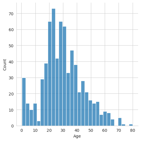
First, let’s visualize the distribution of Age to understand it’s importance:

sns.displot(trn_df['Age'], kde=False, bins=30)

As you can see from the plot Age is one of the most crucial features. Younger passengers had a higher chance to survival, while older passenger had a low chance. So, we need to handle Age with extra care.

To fill in the missing Age values, we’ll use the technique called K-Nearest Neighbors(KNN) imputation. Here’s how it works:

# Age imputation
age_imputer = KNNImputer(n_neighbors=5)
trn_df["Age"] = age_imputer.fit_transform(trn_df[["Age", "Pclass", "SibSp", "Parch"]])[:, 0]

Here’s the breakdown:

  • We select relevant columns that are likely correlated with Age (Pclass, SibSp, and Parch).
  • The fit_transform method is called on the age_imputer instance, passing these columns.
    • Fit: the imputer calculate the distances between rows based on the selected columns and indentifies the 5 nearest neighbors for each instance with with missing Age values.
    • Transform: For each missing Age value, the imputer calculate the mean age of the 5 nearest neighbors and fills in the missing value with this mean.
  • [:, 0] selects the first columns of the resulting array (the imputed Age, values) and assigns it back to the Age columns trn_df.

And that’s our K-Nearest Neighbors(KNN) imputation in action!

Handling Missing Cabin and Embarked Values

Now, let’s talk about the Cabin column. This column has lot of missing values. and it doesn’t have a significant impact on survival rates. So, we’ll use a simple approach to fill these missing values:

modes = trn_df.mode().iloc[0]
trn_df.fillna(modes, inplace=True)

Here, we’re fillng the missing Cabin and two missing Embarded value with the most frequently occurring value (mode). The mode method in Pandas finds the most common value(s) in DataFrame or Series. If multiple modes exist, it return all of them

Outlier Detection and Handling

Next, let’s inspect the Fare column for any outlier:

trn_df.describe(include=np.number)
PassengerId Survived Pclass Age SibSp Parch Fare
count 891.000000 891.000000 891.000000 891.000000 891.000000 891.000000 891.000000
mean 446.000000 0.383838 2.308642 29.828249 0.523008 0.381594 32.204208
std 257.353842 0.486592 0.836071 13.293378 1.102743 0.806057 49.693429
min 1.000000 0.000000 1.000000 0.420000 0.000000 0.000000 0.000000
25% 223.500000 0.000000 2.000000 22.000000 0.000000 0.000000 7.910400
50% 446.000000 0.000000 3.000000 30.000000 0.000000 0.000000 14.454200
75% 668.500000 1.000000 3.000000 35.800000 1.000000 0.000000 31.000000
max 891.000000 1.000000 3.000000 80.000000 8.000000 6.000000 512.329200

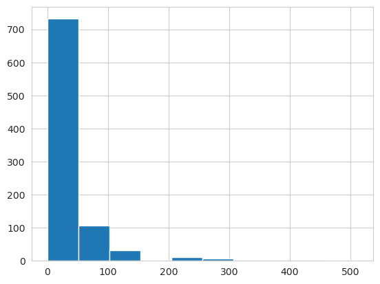
You’ll notice that the mean fare is around 32, but he maximum values is a Whopping 512.3292. Such extreme values can cause issues for our model because they can dominate the results. Let’s visualize this with a histogram:

trn_df['Fare'].hist();

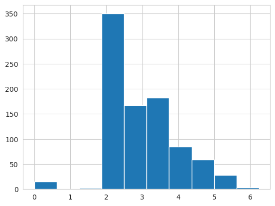
To fix this, we can take the logarithm of the Fare values, which heps to compress the range and make the distribution more reasonable. Since the Fare column contains zeros and log(0) is undefined, we’ll add 1 to all values before applying the logarithm

trn_df["LogFare"] = np.log1p(trn_df['Fare'])
trn_df['LogFare'].hist();

Alright it’s look better now!

And that’s it for data cleaning! We’ve handled missing values and outliers, setting the stage for effective model training, Next up, we’ll dive into feature engineering, whish is where the fun really begins!

Feature Engineering

Alright, buckle up ’cause we’re about to embark on a feature engineering adventure!

First up, we’re gonna create a super coll FamilySize feature. Why? because family matter, especially when you’re trying to survive a shipwreck!

trn_df["FamilySize"] = trn_df["SibSp"] + trn_df["Parch"] + 1
trn_df["IsAlone"] = (trn_df["FamilySize"] == 1).astype(int)

Now, let’s visualize this bad boy:

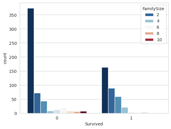
sns.countplot(x='Survived', data=trn_df, hue='FamilySize', palette='RdBu_r')

Whoa, check out that plot! It’s like a family reunion, but with survival rates. Looks like having a big family might’ve been a bit of bummer for survival chances. Maybe it was harder to round up the whole crew when things got dicey? On the flip side, small families (up to 4 members) seemed to have better luck. Family-sized life rafts, perhaps?

Next up, we’re gonna play “Name That Title”!

# Extract title from name
trn_df['Title'] = trn_df['Name'].str.extract(r' ([A-Za-z]+)\.', expand=False)
# Group uncommon titles
rare_titles = ['Lady', 'Countess','Capt', 'Col', 'Don', 'Dr', 'Major', 'Rev', 'Sir', 'Jonkheer', 'Dona']
trn_df['Title'] = trn_df['Title'].replace(rare_titles, 'Rare')
# Replace some variations
trn_df['Title'] = trn_df['Title'].replace(['Mlle', 'Ms'], 'Miss')
trn_df['Title'] = trn_df['Title'].replace('Mme', 'Mrs')
# Mapping
title_mapping = {"Mr": 1, "Miss": 2, "Mrs": 3, "Master": 4, "Rare": 5}
trn_df['Title'] = trn_df['Title'].map(title_mapping)

We’re extracting titles faster than you can say “I’m the king of the world!” We’ve got our common title, we’re grouping the rare ones(because being a Countess doesn’t help much when the ship’s going down), and we’re doing a little title cleanup.

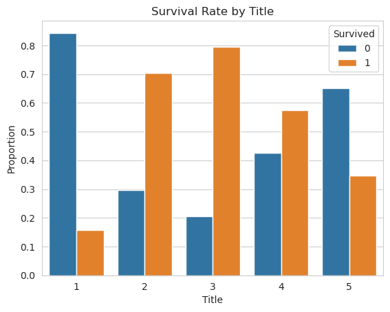
Now, let’s see what these titles tell us about survival:

# Calculate proportions
proportions = trn_df.groupby('Title')['Survived'].value_counts(normalize=True).rename('proportion').reset_index()

sns.barplot(x='Title', y='proportion', hue='Survived', data=proportions)
plt.title('Survival Rate by Title')
plt.xlabel('Title')
plt.ylabel('Proportion')
plt.show()

Holy shipwreck, Batman! look at those survival rates! Poor Mr.1 is going down with the ship, while Mss 2 and Mrs. 3 are living the best lifeboat life.

It captures important historical context about the Titanic disaster, particularly the “women and children first” policy during evacuation.

When we use this feature in our model, it should be able to learn these different survival probabilities associated with each title, potentially improving its predictive accuracy.

Next, we’re gonna group these passengers by age

trn_df['AgeBin'] = pd.cut(trn_df['Age'], bins=[0, 12, 20, 40, 60, np.inf], labels=[1, 2, 3, 4, 5])

and for our grand finale, we’re gonna one-hot encode these categorical columns:

# one hot encode columns
trn_df = pd.get_dummies(trn_df, columns=["Sex", "Pclass", "Embarked", "AgeBin"], drop_first=True, dtype=float)

Alright that’s it, let’s write a function to do all of this for the life easier, because we also need to apply it to our test set so that we can make a proper prediction

def preprocess_data(df):
    age_imputer = KNNImputer(n_neighbors=5)
    df["Age"] = age_imputer.fit_transform(df[["Age", "Pclass", "SibSp", "Parch"]])[:, 0]
    modes = trn_df.mode().iloc[0]
    trn_df.fillna(modes, inplace=True)
    df["LogFare"] = np.log1p(df["Fare"])
    df["FamilySize"] = df["SibSp"] + df["Parch"] + 1
    df['IsAlone'] = (df['FamilySize'] == 1).astype(int)
    df['Title'] = df['Name'].str.extract(r' ([A-Za-z]+)\.', expand=False)
    rare_titles = ['Lady', 'Countess','Capt', 'Col', 'Don', 'Dr', 'Major', 'Rev', 'Sir', 'Jonkheer', 'Dona']
    df['Title'] = df['Title'].replace(rare_titles, 'Rare')
    df['Title'] = df['Title'].replace(['Mlle', 'Ms'], 'Miss')
    df['Title'] = df['Title'].replace('Mme', 'Mrs')
    title_mapping = {"Mr": 1, "Miss": 2, "Mrs": 3, "Master": 4, "Rare": 5}
    df['Title'] = df['Title'].map(title_mapping)
    df['AgeBin'] = pd.cut(df['Age'], bins=[0, 12, 20, 40, 60, np.inf], labels=[1, 2, 3, 4, 5])
    
    # One-hot encoding
    df = pd.get_dummies(df, columns=['Sex', 'Pclass', 'Embarked', 'AgeBin'], drop_first=True, dtype=float)
    return df

Finally, let’s round up our feature posse:

def get_columns(name):
    return [col for col in trn_df.columns if col.startswith(name)]
added_cols = get_columns(("Sex_", "Pclass", "Embarked_", "AgeBin_"))

indep_cols = ['Title', 'Age', 'SibSp', 'Parch', 'LogFare', 'FamilySize', 'IsAlone'] + added_cols
t_dep = tensor(trn_df["Survived"])

And there you have it, folks! We’ve engineeried these features faster than the Titanic sank(too soon?). Your models gonna love these new features more than Rose loved Jack. Now go forth and predict those survival rates!

Build a Deep Learning Model from Scratch: Let’s Get Our Hands Dirty!

Preparing the Canvas

Alright, folks! Before we dive into the exciting world of deep learning, we need to prepare our data. It’s like setting up our art studio before creating a masterpiece. Let’s take a look at what we’re working with:

t_indep = trn_df[indep_cols].values
t_indep
array([[ 1. , 22. ,  1. , ...,  1. ,  0. ,  0. ],
       [ 3. , 38. ,  1. , ...,  1. ,  0. ,  0. ],
       [ 2. , 26. ,  0. , ...,  1. ,  0. ,  0. ],
       ...,
       [ 2. , 28.8,  1. , ...,  1. ,  0. ,  0. ],
       [ 1. , 26. ,  0. , ...,  1. ,  0. ,  0. ],
       [ 1. , 32. ,  0. , ...,  1. ,  0. ,  0. ]])

Whoa there! If you peek at t_indep, you’ll notice something funky. The age columns is partying way to hard compared to it’s friends. This could through our model for a loop, so let’s calm it down a bit

Now, we could go old school and divide each column by its maximum value. It’s like telling your loudest friend to use their indoor voice. The formula would look something like this:

\(Normalized\ value = \frac{Feature\ value} {Maximum\ value\ of\ that\ feature}\)

But hey, we’re not here to play it safe! We’re going to use a cool trick called StandardScaler. It’s like giving each feature i’s own personal stylist. Here’s the magic behind it:

\(z = \frac{x - \mu}{\sigma}\)

Where:

  • \(x\) is the original feature value.
  • \(\mu\) is the mean of the feature values.
  • \(\sigma\) is the standard deviation of the feature values.
  • \(z\) is the standardized value.

Why StandardScaler, you ask? Well, it’s got some neat perks:

  1. It handles outliers like a boss. Max scaling can sometimes squish all your other values when one outliers decides to go crazy.
  2. it’s a gradient descent’s best friend. when you’re dealing with neural networks, having features one a similar scale is like having a smooth road for your optimization on cruise on.

Let’s wave our magic wand and see what happens:

scaler = StandardScaler()
t_indep = tensor(scaler.fit_transform(t_indep), dtype=torch.float)
#dependent variable
t_dep = tensor(trn_df['Survived'].values)
t_indep
tensor([[-0.7076, -0.5892,  0.4328, -0.4737, -0.8797,  0.0592, -1.2316,  ...,  0.9026, -0.3076,  0.6158, -0.3753,  0.7874, -0.4115,
         -0.1591],
        [ 1.2352,  0.6151,  0.4328, -0.4737,  1.3612,  0.0592, -1.2316,  ..., -1.1079, -0.3076, -1.6238, -0.3753,  0.7874, -0.4115,
         -0.1591],
        [ 0.2638, -0.2881, -0.4745, -0.4737, -0.7985, -0.5610,  0.8119,  ...,  0.9026, -0.3076,  0.6158, -0.3753,  0.7874, -0.4115,
         -0.1591],
        [ 1.2352,  0.3893,  0.4328, -0.4737,  1.0620,  0.0592, -1.2316,  ..., -1.1079, -0.3076,  0.6158, -0.3753,  0.7874, -0.4115,
         -0.1591],
        [-0.7076,  0.3893, -0.4745, -0.4737, -0.7842, -0.5610,  0.8119,  ...,  0.9026, -0.3076,  0.6158, -0.3753,  0.7874, -0.4115,
         -0.1591],
        [-0.7076,  0.2312, -0.4745, -0.4737, -0.7386, -0.5610,  0.8119,  ...,  0.9026,  3.2514, -1.6238, -0.3753,  0.7874, -0.4115,
         -0.1591],
        [-0.7076,  1.8194, -0.4745, -0.4737,  1.0381, -0.5610,  0.8119,  ..., -1.1079, -0.3076,  0.6158, -0.3753, -1.2700,  2.4304,
         -0.1591],
        ...,
        [-0.7076, -0.3634, -0.4745, -0.4737, -0.9051, -0.5610,  0.8119,  ...,  0.9026, -0.3076,  0.6158, -0.3753,  0.7874, -0.4115,
         -0.1591],
        [ 1.2352,  0.6903, -0.4745,  5.7328,  0.4575,  2.5397, -1.2316,  ...,  0.9026,  3.2514, -1.6238, -0.3753,  0.7874, -0.4115,
         -0.1591],
        [ 3.1780, -0.2129, -0.4745, -0.4737, -0.3337, -0.5610,  0.8119,  ..., -1.1079, -0.3076,  0.6158, -0.3753,  0.7874, -0.4115,
         -0.1591],
        [ 0.2638, -0.8150, -0.4745, -0.4737,  0.4871, -0.5610,  0.8119,  ..., -1.1079, -0.3076,  0.6158,  2.6646, -1.2700, -0.4115,
         -0.1591],
        [ 0.2638, -0.0774,  0.4328,  2.0089,  0.2420,  1.2994, -1.2316,  ...,  0.9026, -0.3076,  0.6158, -0.3753,  0.7874, -0.4115,
         -0.1591],
        [-0.7076, -0.2881, -0.4745, -0.4737,  0.4871, -0.5610,  0.8119,  ..., -1.1079, -0.3076, -1.6238, -0.3753,  0.7874, -0.4115,
         -0.1591],
        [-0.7076,  0.1635, -0.4745, -0.4737, -0.8190, -0.5610,  0.8119,  ...,  0.9026,  3.2514, -1.6238, -0.3753,  0.7874, -0.4115,
         -0.1591]])
Look at that! Our t_indep is now looking sharp and ready for action.

But wait, there’s more! We’re going to split our data into a training set and a validation set. Sure, our dataset might be on the smaller side, but having a validation set is like having a trusty sidekick. It’s helps us keep an eye on our model’s performance and prevents it from getting too cocky (aka overfitting). We’ll use the RandomSplitter in the fastai library to split our dataset

torch.manual_seed(442)
from fastai.data.transforms import RandomSplitter
trn_split, val_split = RandomSplitter(seed=42)(trn_df)

trn_indep, val_indep = t_indep[trn_split], t_indep[val_split]
trn_dep, val_dep = t_dep[trn_split], t_dep[val_split]

And there you have it, folks! We’ve got everything we need to start our training montage. Get ready, because we’re about to embark on a wild ride through the world of deep learning. It’s gooing to be a fun one!

The Model Architecture: Our Neural Blueprint

First things first, let’s create a a function to initialize our coefficients. Think of this as laying the foundation for our neural masterpiece

def init_coeffs(n_input, n_hidden=10):
    torch.manual_seed(442)
    layer_1 = torch.randn(n_input, n_hidden) / np.sqrt(n_input)
    layer_2 = torch.randn(n_hidden, 1) / np.sqrt(n_hidden)
    const = torch.rand(1)[0]
    return (layer_1.requires_grad_(), layer_2.requires_grad_(), const.requires_grad_())

Now, you might wondering, “Why only one hidden layer with 10 units?” Well, my friends, sometimes less is more? With a small dataset like Titanic, a simple architecture often works best - compact but effective!

But wait, what’s with tat square root division? Great question! It’s all about keeping our neural network balanced. By dividing by the square root of inputs, we’re making sure our data doesn’t go haywire as it flows through the network. It’s like adding just the right amount of spice to your cooking - not too much - not too little!

Next up, let’s write a function to calculate our predictions:

def calc_preds(coeffs, indep):
    l1, l2, const = coeffs
    res = F.relu(indep @ l1) 
    res = res@l2 + const
    return torch.sigmoid(res)

This is where magic happens! We’re using matrix multiplication (that’s what the @ symbol does) and applying our good friend RelLU. Remember our chat about ReLU earlier? This is where it comes into play! If you want to dive deeper into the power of ReLU, check out my previous blog post here.

Now, let’s talk about loss. No, not the kind you feel when MU loses, but the kind that tells use how well our model is doing:

def calc_loss(coeffs, indeps, deps):
    return torch.abs(calc_preds(coeffs, indeps)-deps.float().unsqueeze(1)).mean()

We’re using mean absolute error here. It’s like measuring how far off our guess are from the real answers and taking the average. Simple, but effective!

Alright, now for the main event - What happens in one epoch of training:

def one_epoch(coeffs, lr, batch_size=64):
    n = len(trn_indep)
    for i in range(0, n, batch_size):
        batch_indep = trn_indep[i:i+batch_size]
        batch_dep = trn_dep[i:i+batch_size]
        
        loss = calc_loss(coeffs, batch_indep, batch_dep)
        loss.backward()

        with torch.no_grad():
            for layer in coeffs:
                layer.sub_(layer.grad * lr)
                layer.grad.zero_()

This is where we use the mini-batch technique. It’s like learning from a small group of examples at a time instead of trying to memorize the whole text book at one. It’s more efficient and helps our model learn better!

Finally, let’s put it all together in our training function:

def train_model(epochs=300, lr=0.01):
    torch.manual_seed(442)
    coeffs = init_coeffs(trn_indep.shape[1])
    best_val_loss = float("inf")
    patience = 20
    counter = 0

    for epoch in range(epochs):
        one_epoch(coeffs, lr)
        with torch.no_grad():
            train_loss = calc_loss(coeffs, trn_indep, trn_dep)
            val_loss = calc_loss(coeffs, val_indep, val_dep)
        
        if val_loss < best_val_loss:
            best_val_loss = val_loss
            best_coeffs = [c.clone() for c in coeffs]
            counter = 0
        else:
            counter += 1
        
        if counter > patience:
            print(f"Early stopping at epoch {epoch}")
            break

        if epoch % 5 == 0:
            print(f"Epoch {epoch}: Train Loss {train_loss:.4f}, Val Loss {val_loss:.4f}")
        lr *= 0.97  # learning rate schedule
    return best_coeffs

This function is like the conductor of our neural orchestra. It initializes our model, trains it for a number of epochs, and learning rate scheduling (to help our model converge more precisely).

And there you have it, folks! We’ve built a neural network from scratch. It might not look like much, but this little guy is ready to tackle the Titanic competition. In our next post, we’ll put it to the test and see how it performs.

Evaluation and Submission: the Moment of Truth!

Alright, folks, it’s time to put our homemade neural network to the test! Let’s see how well it can predict who survived the Titanic disaster.

First, we need a way to measure our model’s performance. Here’s our accuracy function:

# Evaluate the model
def acc(coeffs): 
    return (val_dep.bool() == (calc_preds(coeffs, val_indep) > 0.5).squeeze()).float().mean()

This function compare our model’s predictions with the actual survival outcomes and calculates the percentage of correct guesses. Simple, but effective!

Now, let’s train our model and see how it performs:

coeffs = train_model(epochs=50, lr=1) 
print(f"Validation Accuracy: {acc(coeffs):.4f}")
Epoch 0: Train Loss 0.3485, Val Loss 0.3620
Epoch 5: Train Loss 0.1921, Val Loss 0.1934
Epoch 10: Train Loss 0.1819, Val Loss 0.1850
Epoch 15: Train Loss 0.1775, Val Loss 0.1805
Epoch 20: Train Loss 0.1739, Val Loss 0.1783
Epoch 25: Train Loss 0.1715, Val Loss 0.1771
Epoch 30: Train Loss 0.1702, Val Loss 0.1759
Epoch 35: Train Loss 0.1693, Val Loss 0.1750
Epoch 40: Train Loss 0.1686, Val Loss 0.1744
Epoch 45: Train Loss 0.1680, Val Loss 0.1741
Validation Accuracy: 0.8315

And the results are in!

Well, well, well! look at that! our little neural network is showing some serious potential. We’re seeing the losses decrease over time for both our training and validation sets, which is exactly what we want. It means our model is learning!

And that validation accuracy? 83.15%! Not too shabby for a model we built from scratch, right? In the world of the Titanic competition, that’s a pretty solid score.(not count those who use extra data to train their model, we all know that).

But the real test is yet to come. How will our model perform on the unseen test data? Let’s find out!

After preprocessing our test data(just like we did with our trainding data), we make our predictions:

## Load and preprocess test data
test_df = pd.read_csv(path / "test.csv")
test_df['Fare'] = test_df.Fare.fillna(0)
test_df = preprocess_data(test_df)

tst_indep = torch.tensor(test_df[indep_cols].values, dtype=torch.float)
# Scale test data using the same scaler
tst_indep = torch.tensor(scaler.transform(tst_indep), dtype=torch.float)

# Make predictions
test_df['Survived'] = (calc_preds(coeffs, tst_indep)>0.5).int()

Let’s take a quick look at our predictions:

sub_df = test_df[['PassengerId', 'Survived']]
print(sub_df["Survived"].sum())
print(sub_df["Survived"].value_counts())
149
Survived
0    269
1    149
Name: count, dtype: int64

Interesting! Our model predicts that 149 passengers survived the Titanic disaster. This about 35.6% of the test set, which is pretty close to the actual survival rate of the Titanic (about 32%). It’s a good sign that our model isn’t wildly off in its predictions.

Now for the moment of truth - submitting to Kaggle!

if you have kaggle api you can use this command

kaggle competitions submit -c titanic -f sub.csv -m "submit to competition"

or you can upload the csv file manual in the competition submit page

AFter submitting, we got anaccuracy of 0.77751% on the test set. That’s 77.75% accuracy on unseen data! For a first attempt with a model we built from scratch, that’s pretty impressive. We’re definitely in the right track!

While 77.75% accuracy is great start, there’s always rooms for improvement. Let’s see if we can push our accuracy even higher.

Leveling Up Our Neural Network: The Pytorch Edition!

Alright, Neural network enthusiasts! We’ve had some success with our homemade model, but now it’s time to kick things up a notch. We’re going to harness the power or Pytorch to create a slightly more sophisticated neural network. Buckle up, because this is where things get exciting!

already let’s write our new architecture.

class SimpleNN(torch.nn.Module):
    def __init__(self, input_size, hidden_size):
        super(SimpleNN, self).__init__()
        self.fc1 = torch.nn.Linear(input_size, hidden_size)
        self.bn1 = torch.nn.BatchNorm1d(hidden_size)
        self.fc2 = torch.nn.Linear(hidden_size, 1)
    
    def forward(self, x):
        x = F.relu(self.bn1(self.fc1(x)))
        x = torch.sigmoid(self.fc2(x))
        return x

This little beauty is like our previous model’s cooler, more sophisticated cousin. It’s still simple, but it’s packing some extra punch:

  • We’ve got two fully connected layers (fc1 and fc2), just like before.
  • But wait, what’s that bn1? That’s batch normalization layer! it’s like traffic cop for our data, making sure everything flows smoothly between layers.
  • We’re still using ReLU and sigmoid activations, because hey, if it ain’t broke, don’t fix it!

Training Our New Model: The Pytorch Way

Now, let’s look at our sniny new training function:

def train_model(model, X_train, y_train, X_val, y_val, epochs=300, lr=0.01, batch_size=32):
    optimizer = torch.optim.Adam(model.parameters(), lr=lr, weight_decay=0.01)  # L2 regularization
    scheduler = torch.optim.lr_scheduler.StepLR(optimizer, step_size=50, gamma=0.5)  # Step LR schedule
    
    best_val_loss = float('inf')
    patience = 20
    counter = 0
    
    for epoch in range(epochs):
        model.train()
        for i in range(0, len(X_train), batch_size):
            batch_X = X_train[i:i+batch_size]
            batch_y = y_train[i:i+batch_size]
            
            optimizer.zero_grad()
            outputs = model(batch_X)
            loss = F.binary_cross_entropy(outputs, batch_y.unsqueeze(1))
            loss.backward()
            optimizer.step()
        
        scheduler.step()
        
        model.eval()
        with torch.no_grad():
            val_outputs = model(X_val)
            val_loss = F.binary_cross_entropy(val_outputs, y_val.unsqueeze(1))
            
        if val_loss < best_val_loss:
            best_val_loss = val_loss
            best_model = model.state_dict()
            counter = 0
        else:
            counter += 1
        
        if counter > patience:
            print(f"Early stopping at epoch {epoch}")
            break
        
        if epoch % 10 == 0:
            print(f"Epoch {epoch}: Train Loss {loss.item():.4f}, Val Loss {val_loss.item():.4f}")
    
    model.load_state_dict(best_model)
    return model

This function is like a personal trainer for our model. Here’s what’s new:

  • We’re using Adam optimizer - it’s like giving our model a smart personal coach that adapts the trainign intensity for each parameter and ’cause this post is a bit too long so i think i will explain Adam optimizer in the different blog post.
  • We’ve added a learning rate scheduler. It’s like adjusting the difficulty of our model’s workout every 50 epochs. Maybe i’ll explain this in another blog post too, it worth an blog post to talk about this.
  • We’re using binary cross-entropy loss now, which is perfect for our binary classification problem.

Now, we have the forward pass:

optimizer.zero_grad()
outputs = model(batch_X)
loss = F.binary_cross_entropy(outputs, batch_y.unsqueeze(1))
loss.backward()
optimizer.step()

This is where the real learning happens:

  1. We clear out any leftover gradients with optimizer.zero_grad(). It’s like wiping the whiteboard clean before a new lesson.

  2. outputs = model(batch_X) it our model making it’s best guess based on what it know so far.

  3. We calculate how wrong we were with loss = F.binary_cross_entropy(...). this is like getting our test results back

  4. Finally, optimizer.step() applies these adjustments. it’s like making notes on how to improve for the next test

After each epoch, we adjust our learning rate:

scheduler.step()

this is like adjusting the difficulty as we get better. We don’t want things to be too easy or too hard!

Lastly, we check how we’re doing on the validation set:

model.eval()
with torch.no_grad():
    val_outputs = model(X_val)
    val_loss = F.binary_cross_entropy(val_outputs, y_val.unsqueeze(1))

this is just as before so nothing to explain here alright

alright let’s put our new model through it’s paces:

# Prepare the data
scaler = StandardScaler()
X = scaler.fit_transform(trn_df[indep_cols].values)
y = trn_df['Survived'].values

X_train, X_val, y_train, y_val = train_test_split(X, y, test_size=0.2, random_state=42)

X_train = torch.FloatTensor(X_train)
y_train = torch.FloatTensor(y_train)
X_val = torch.FloatTensor(X_val)
y_val = torch.FloatTensor(y_val)

# Initialize and train the model
input_size = X_train.shape[1]
hidden_size = 10
model = SimpleNN(input_size, hidden_size)

trained_model = train_model(model, X_train, y_train, X_val, y_val, epochs=50, lr=0.02)

# Evaluate the model
model.eval()
with torch.no_grad():
    val_outputs = model(X_val)
    val_preds = (val_outputs > 0.5).float()
    accuracy = (val_preds.squeeze() == y_val).float().mean()
    print(f"Validation Accuracy: {accuracy.item():.4f}")
Epoch 0: Train Loss 0.3662, Val Loss 0.4901
Epoch 10: Train Loss 0.2244, Val Loss 0.4254
Epoch 20: Train Loss 0.2155, Val Loss 0.4271
Early stopping at epoch 29
Validation Accuracy: 0.8268

Our model decided to call it quits after just 29 epochs. Our validation accuracy is …82.68%? That’s actually a bit lower that our previous model. But don’t panic! Sometimes, a slightly lower validation accuracy can lead to better performance on unseen data. It’s like how sometimes taking it easyy in practice can lead to better performance in the big game.

alright let submit to kaggle to see how our model performs on test set, shall we!

## Load and preprocess test data
test_df = pd.read_csv(path / "test.csv")
test_df = preprocess_data(test_df)

# Ensure test_df has all the necessary columns
for col in indep_cols:
    if col not in test_df.columns:
        test_df[col] = 0  # or some appropriate default value

X_test = test_df[indep_cols].values
X_test = scaler.transform(X_test)
X_test = torch.FloatTensor(X_test)

i just did as before

# Make predictions on test set
model.eval()
with torch.no_grad():
    test_outputs = model(X_test)
    test_preds = (test_outputs > 0.5).int()
test_df["Survived"] = test_preds

same thing here

sub_df = test_df[['PassengerId', 'Survived']]
print(sub_df["Survived"].sum())
print(sub_df["Survived"].value_counts())
149
Survived
0    269
1    149
Name: count, dtype: int64

alright everythig seems good till now, let’s make our submit shall we?

sub_df.to_csv("sub_ver3.csv", index=False)
!head sub_ver3.csv
PassengerId,Survived
892,0
893,0
894,0
895,0
896,1
897,0
898,1
899,0
900,1

alright in the time i write this blog post i got this result

we got an accuracy of 0.78708! That’s 78.71%, which is a solid improvement over our previous score of 77.51%. We’ve climbed another rung on the Kaggle leaderboard ladder!

What Have We Learned?

  1. Sometimes, a more complex model (like our PyTorch version) can lead to better generalization, even if the validation accuracy is slightly lower.

  2. Early stopping can prevent overfitting - our model knew when to quit while it was ahead.

  3. Consistency in predictions (149 survivors in both models) suggests we’re on the right track.

Remember, in the world of machine learning as well as deep learning, there’s always room for improvement. So keep experimenting, keep learning, and who knows? Maybe you’ll be the one to finally crack the Titanic code and reach that coveted top spot on the Kaggle leaderboard!

Until next time, happy modeling, and may the gradients be ever in your favor!